8. EXAMPLES

8.1. Example 1 - Spread Footing

8.1.1. Problem Formulation

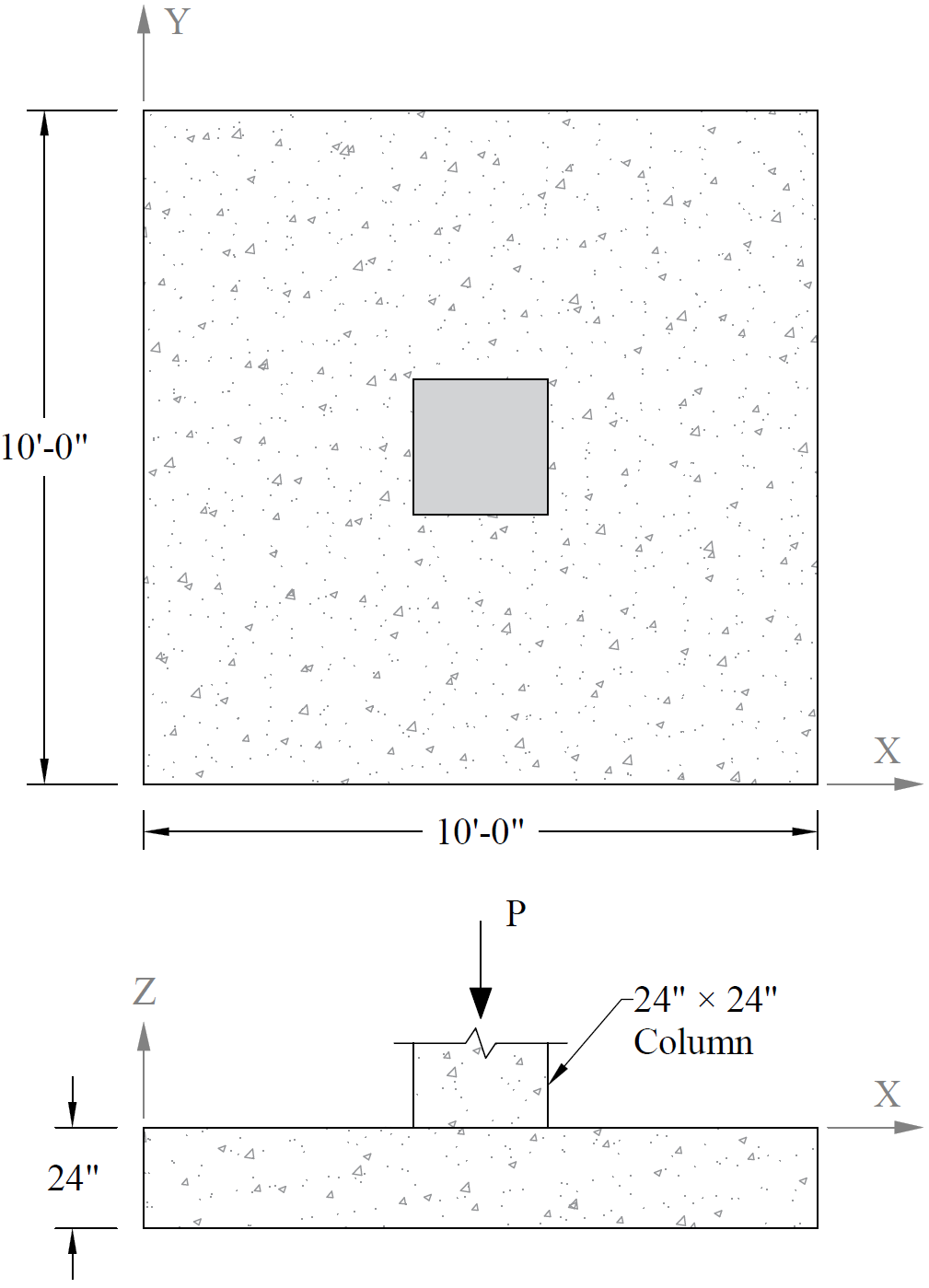
A square footing with dimension 10 ft × 10 ft and a thickness of 2 ft will be analyzed and designed to support a 500 kip axial load applied at its center.¹

Design data

The origin of the XY plane will be located at the lower left-hand corner of the footing. Two-foot square elements will be used.

Column Loading Conditions

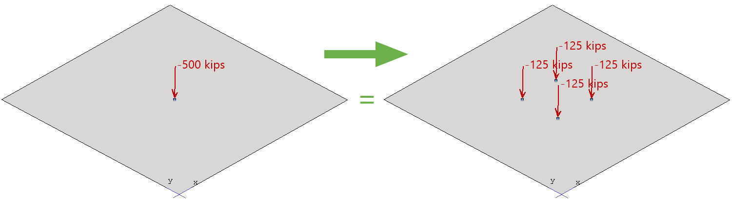
The concentrated load will be applied as four nodal loads (500 kips / 4 = 125 kips per node).

8.1.2. Preparing the Input²

1. From the Start screen, select New Project.

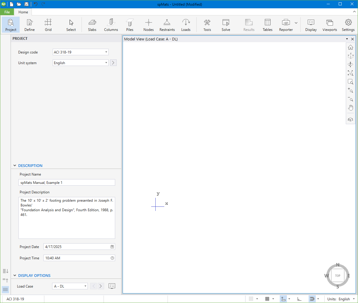
2. In the Main Program Window, select Project from the Ribbon.

• Select the DESIGN CODE, UNIT SYSTEM, and enter the PROJECT NAME and PROJECT DESCRIPTION.

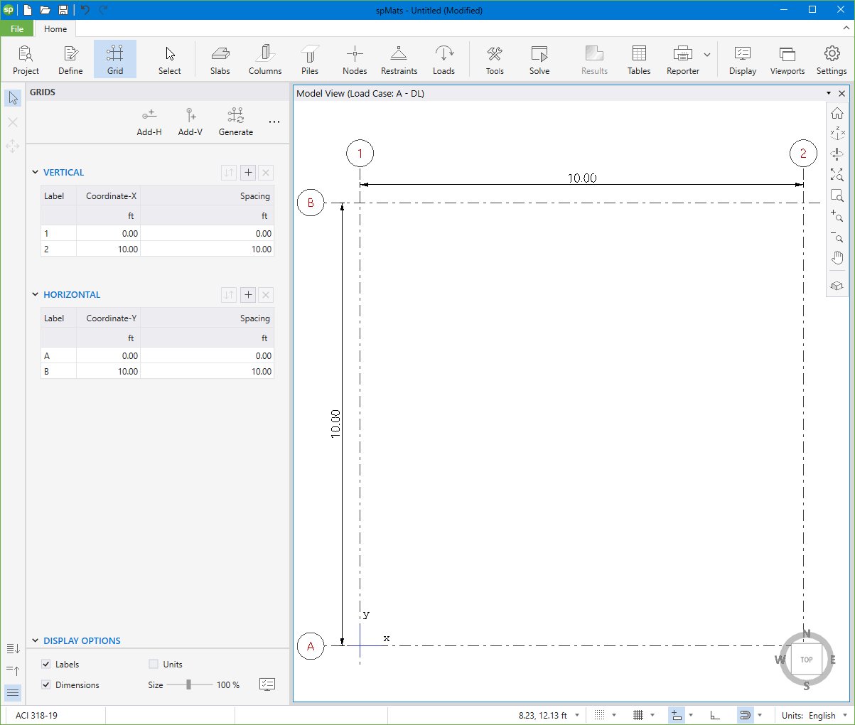
3. From the Ribbon, select Grid.

• Click on the Generate in the left panel to have the program surface the following:

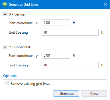
• Place a check mark in the X - VERTICAL box and enter the following values in the corresponding text boxes:

• Place a check mark in the Y - VERTICAL box and enter the following values in the corresponding text boxes:

• Click on the GENERATE button to return to the main window. Notice how the VERTICAL and HORIZONTAL grid lines now appear in the VIEWPORT.

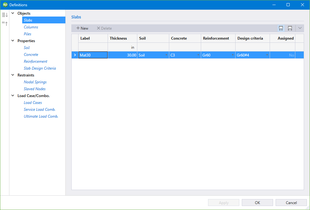
4. From the Ribbon, select Define, then choose Slabs from Objects to display the Slabs dialog box.

• Input Mat30 for LABEL and 30.00 in. for THICKNESS.

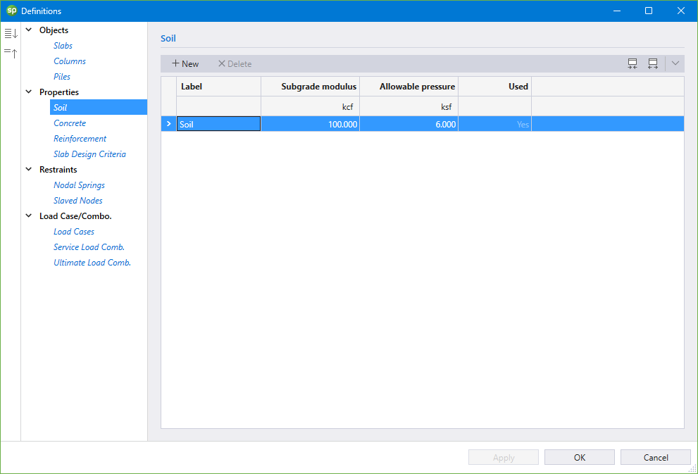
5. Click on Soil from Properties to display the Soil dialog box.

• Enter the following:

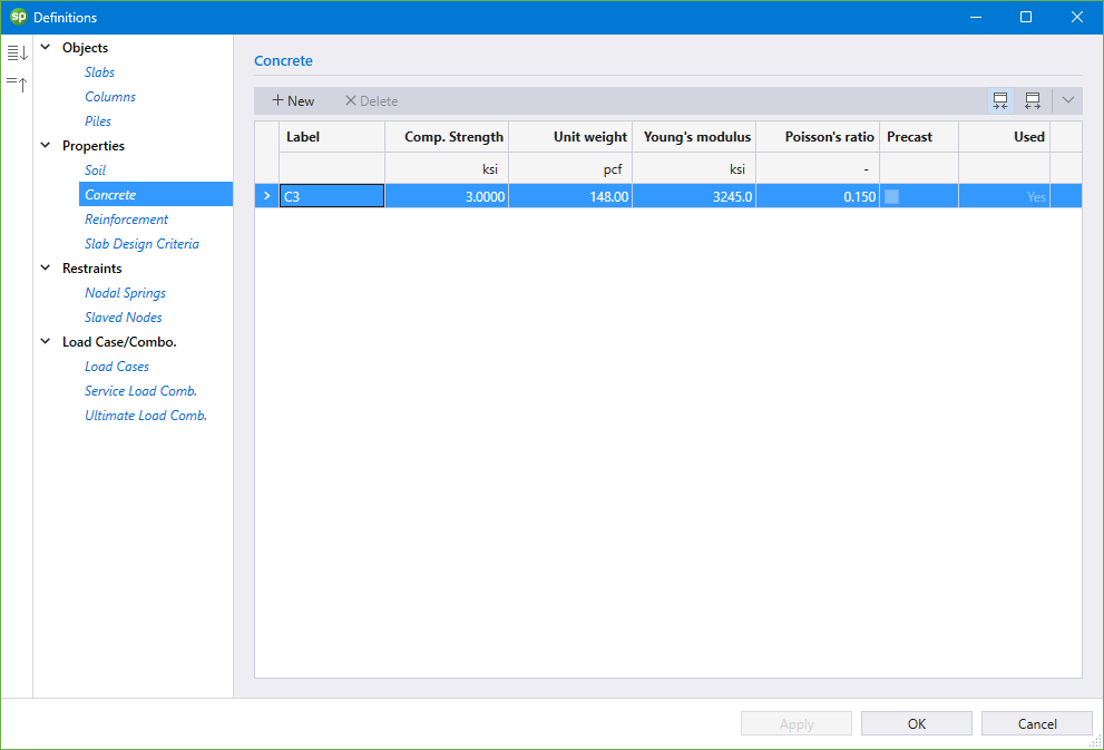
6. Click on Concrete from Properties to display the Concrete dialog box.

• Enter the following:

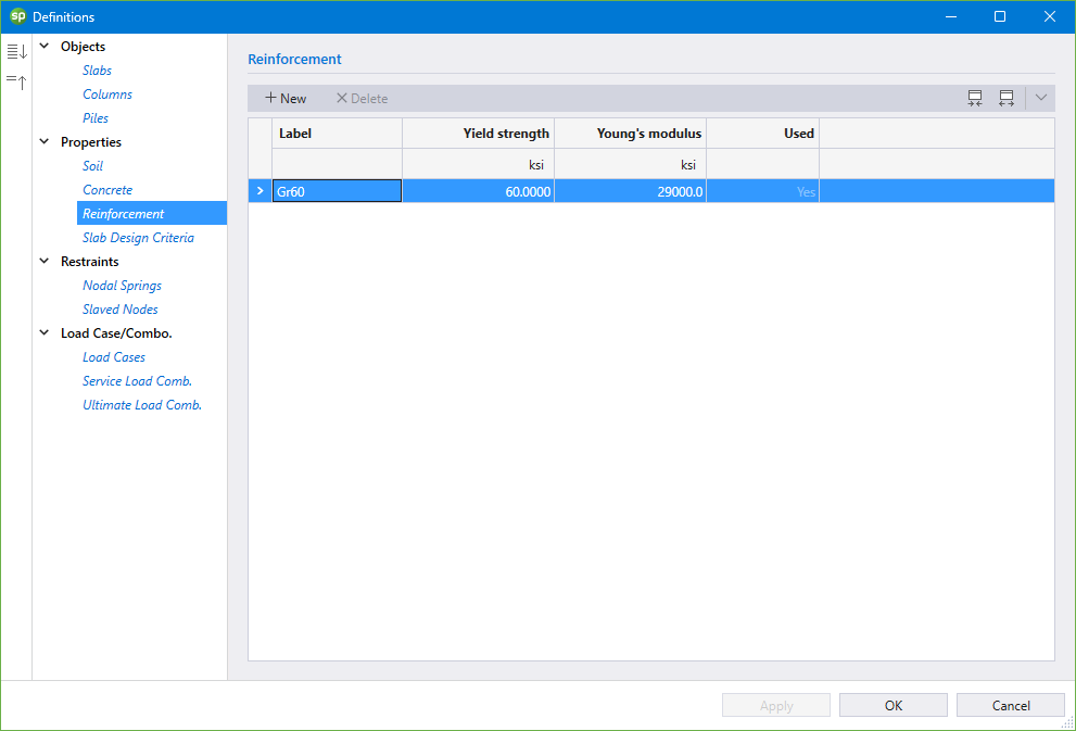
7. Click on Reinforcement from Properties to display the Reinforcement dialog box.

• Enter the following:

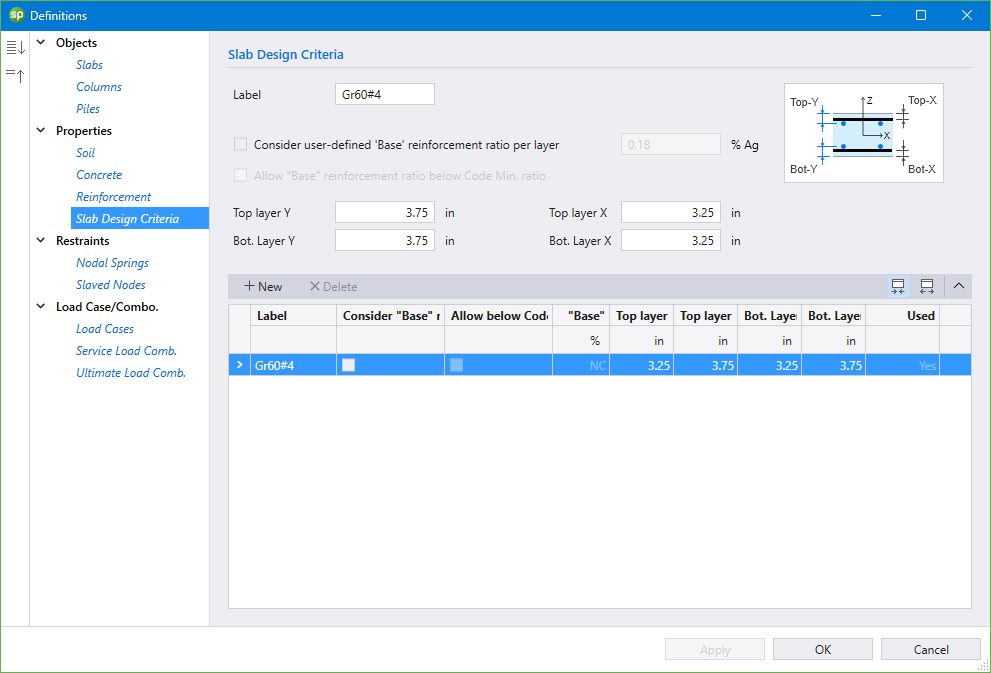
8. Click on Slab Design Criteria from Properties to display the Slab Design Criteria dialog box.

• Enter the following:

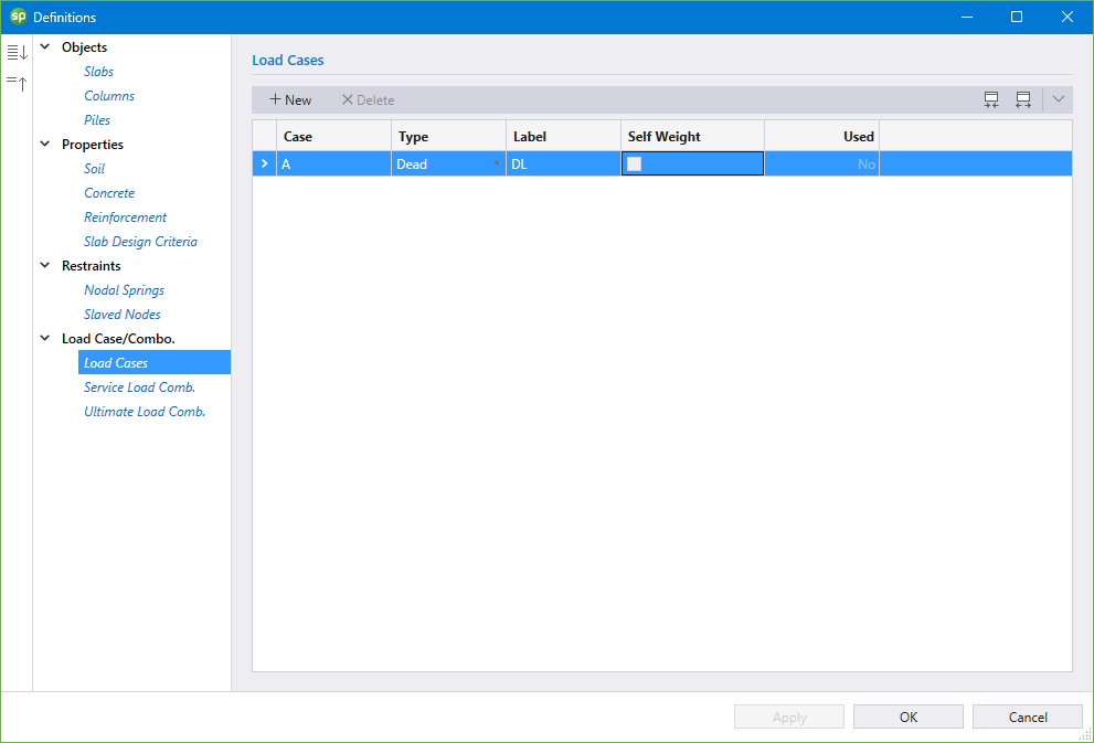
9. Click on Loads Cases from Load Case/Combo. to display the Load Cases dialog box.

• Enter the following:

CASE A: DL

• Uncheck SELF WEIGHT for CASE A.

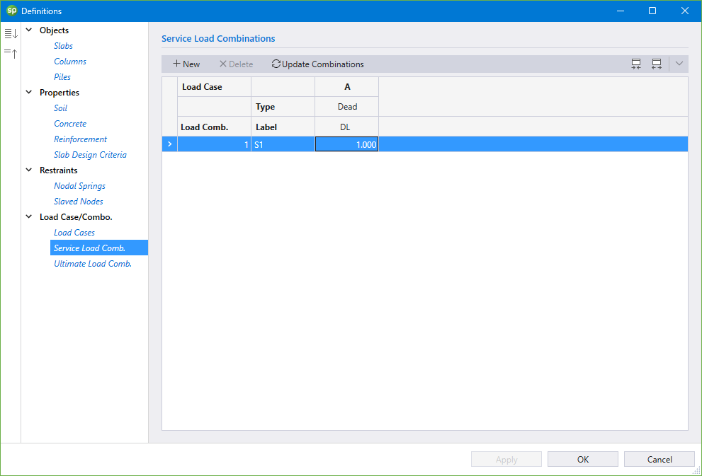
10. Click on Service Load Combinations from Load Case/Combo. to display the Service Load Combinations dialog box.

• Enter the following service load combinations shown in the figure below:

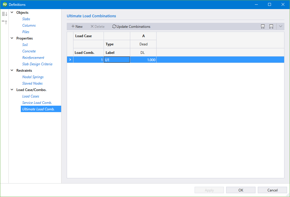
11. Click on Ultimate Load Combinations from Load Case/Combo. to display the Ultimate Load Combinations dialog box.

• Enter the following load combinations shown in the figure below:

8.1.3. Assigning Properties

12. From the Ribbon, select Slabs command.

• In the left panel, select Rectangle then select MAT30 from LABEL.

• In the VIEWPORT, marquee-select the region (A, 1) – (B, 2) to apply the selected slab to the entire foundation.

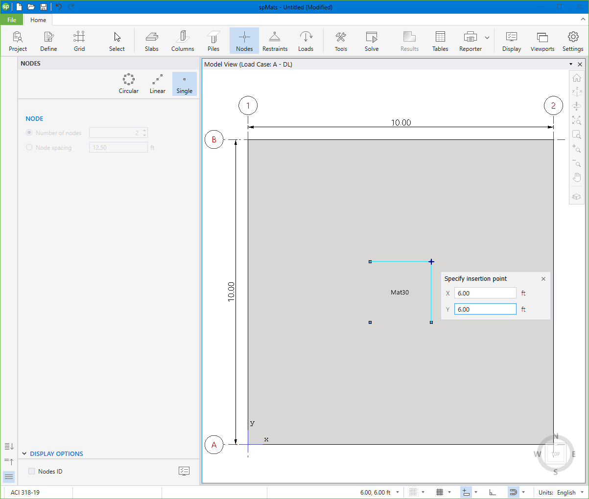
13. From the Ribbon, select Nodes command.

• In the left panel, select Single.

• In the VIEWPORT, enter the coordinates of each node using the dynamic input box (to activate the dynamic input box simply start typing):

NODE 1: (4, 4)

NODE 2: (6, 4)

NODE 3: (4, 6)

NODE 4: (6, 6)

8.1.4. Assigning Loads

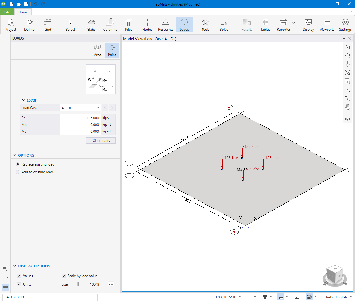
14. From the Ribbon, select Loads command.

• In the left panel, select Point then select A-DL from LOAD CASE and enter the following:

P_Z: -125.00 kips

• Apply to all nodes as shown in the figure below.

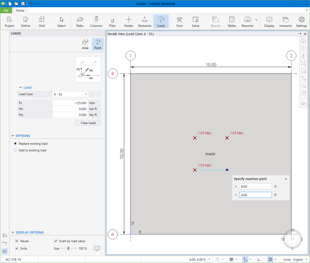
• Also, you can click on the 3D VIEW icon from View Controls (top right of the active viewport) to get a better view of the applied loads.

8.1.5. Solving

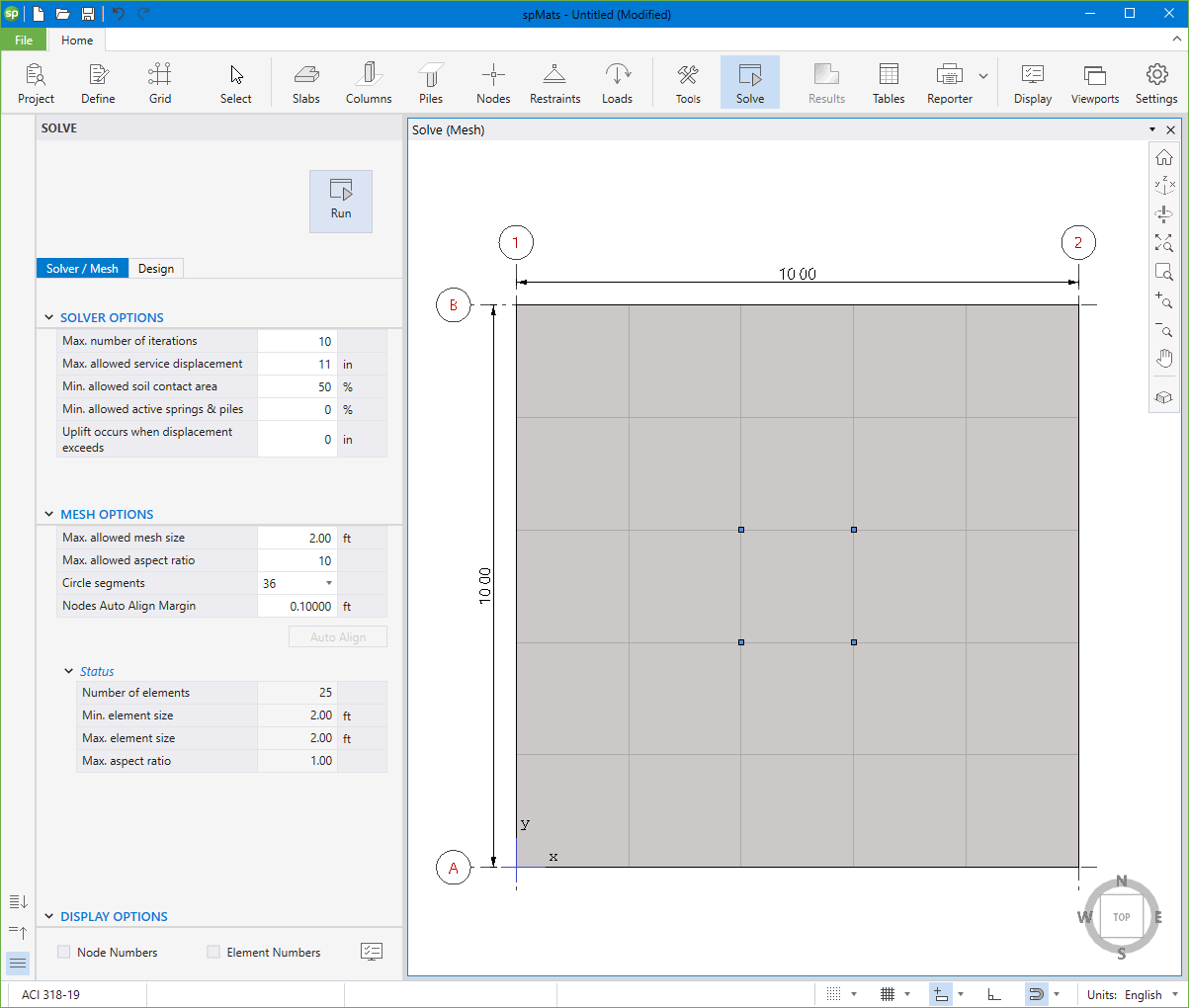
15. From the Ribbon, select Solve command.

For Solver / Mesh Options:

• Leave all Solver Options to their default settings.

• Leave all Mesh Options to their default settings.

For Design Options:

• Leave all Slab Design Options to their default settings.

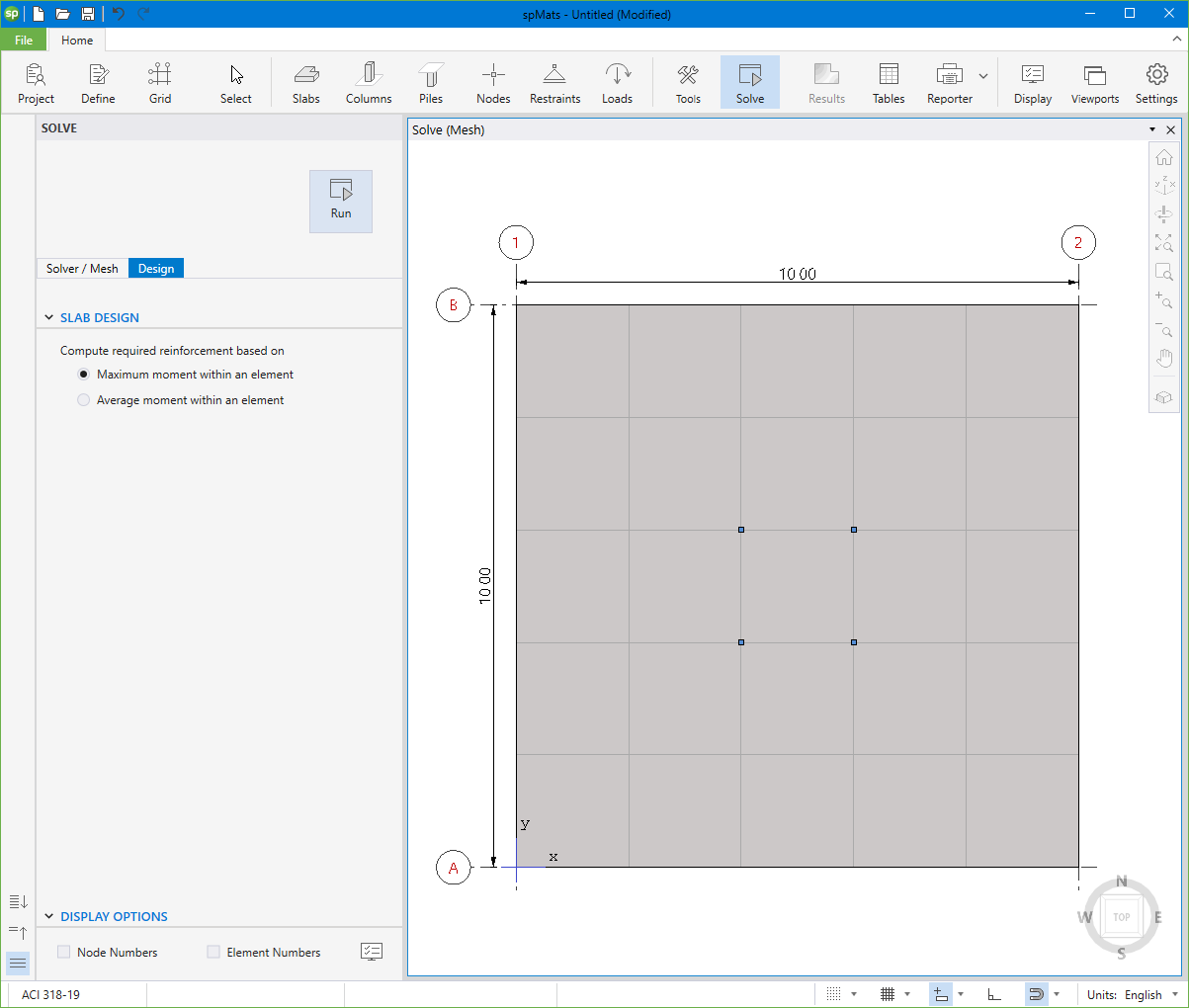
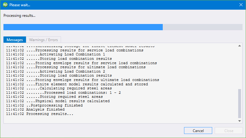
• Click on the Run button.

• The spMats Solver window is displayed and the solver messages are listed. After the solution is done, the design will be performed and then the focus will immediately be passed to the Contours scope.

8.1.6. Viewing and Printing Results

16. After a successful run, results can be viewed in a contour form.

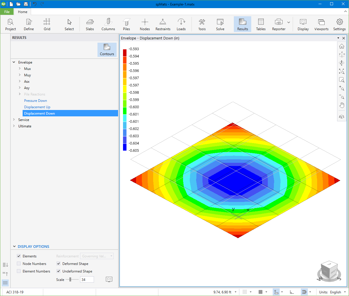
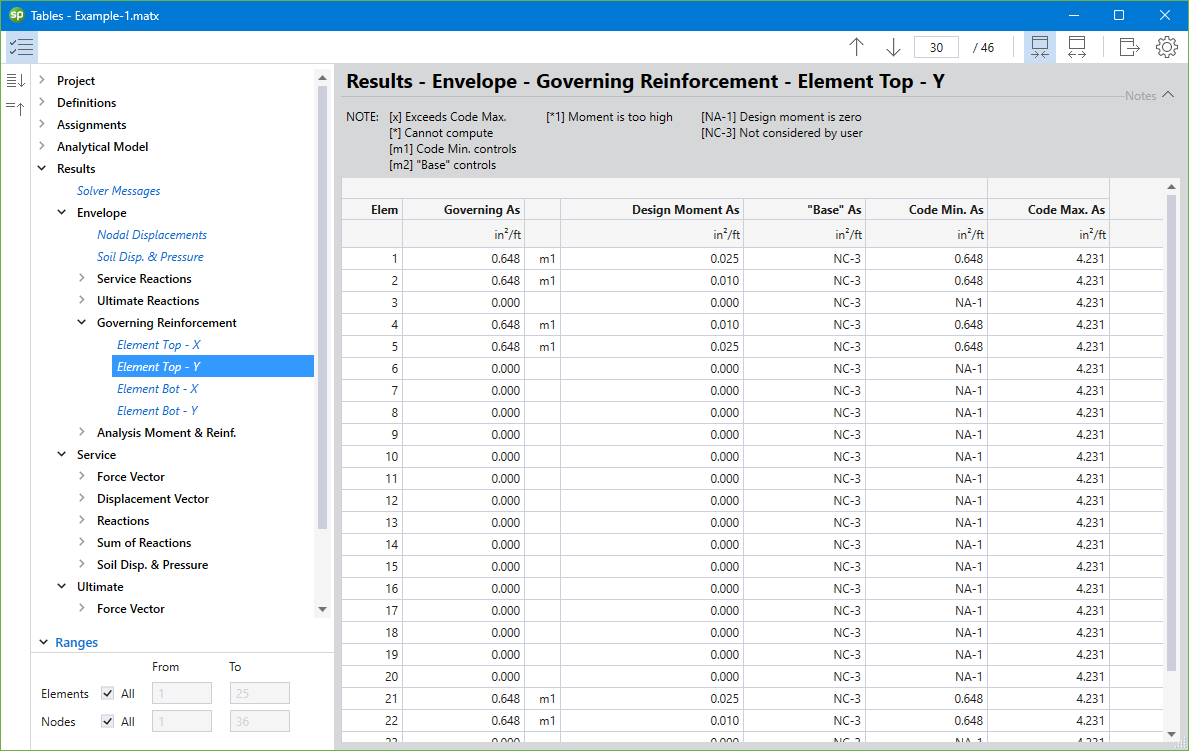
17. Results can be also viewed in table format by selecting the Tables command from the Ribbon.

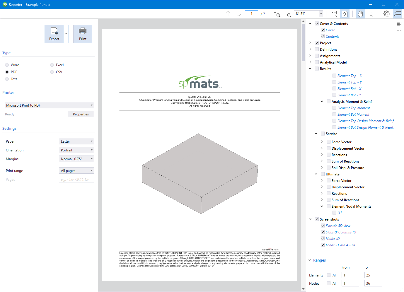
18. Results can be printed or exported in different formats by selecting the Reporter command from the Ribbon.