8. EXAMPLES

8.1. Example 1 - Load Bearing Wall

8.1.1. Problem Formulation

This example will illustrate the analysis and design of the wall shown below. As is required for typical precast or tilt-up load bearing panels, a second order analysis will be performed.

Design data

f_c’ = 4,000 psi

w_c = 150 pcf

v (Poisson’s ratio) = 0.20

f_y = 60,000 psi

E_s = 29,000 ksi

Wall thickness = 8.75 in.

Eccentricity (e) = 7.50 in.

Roof dead load = 0.40 klf (line load)

Roof live load = 0.50 klf (line load)

Wind load = 30.0 psf (uniform area load)

Reinforcement for this wall is considered as two curtains, each composed of two layers: one horizontal with 1 in. cover, and one vertical with 1.5 in. cover.

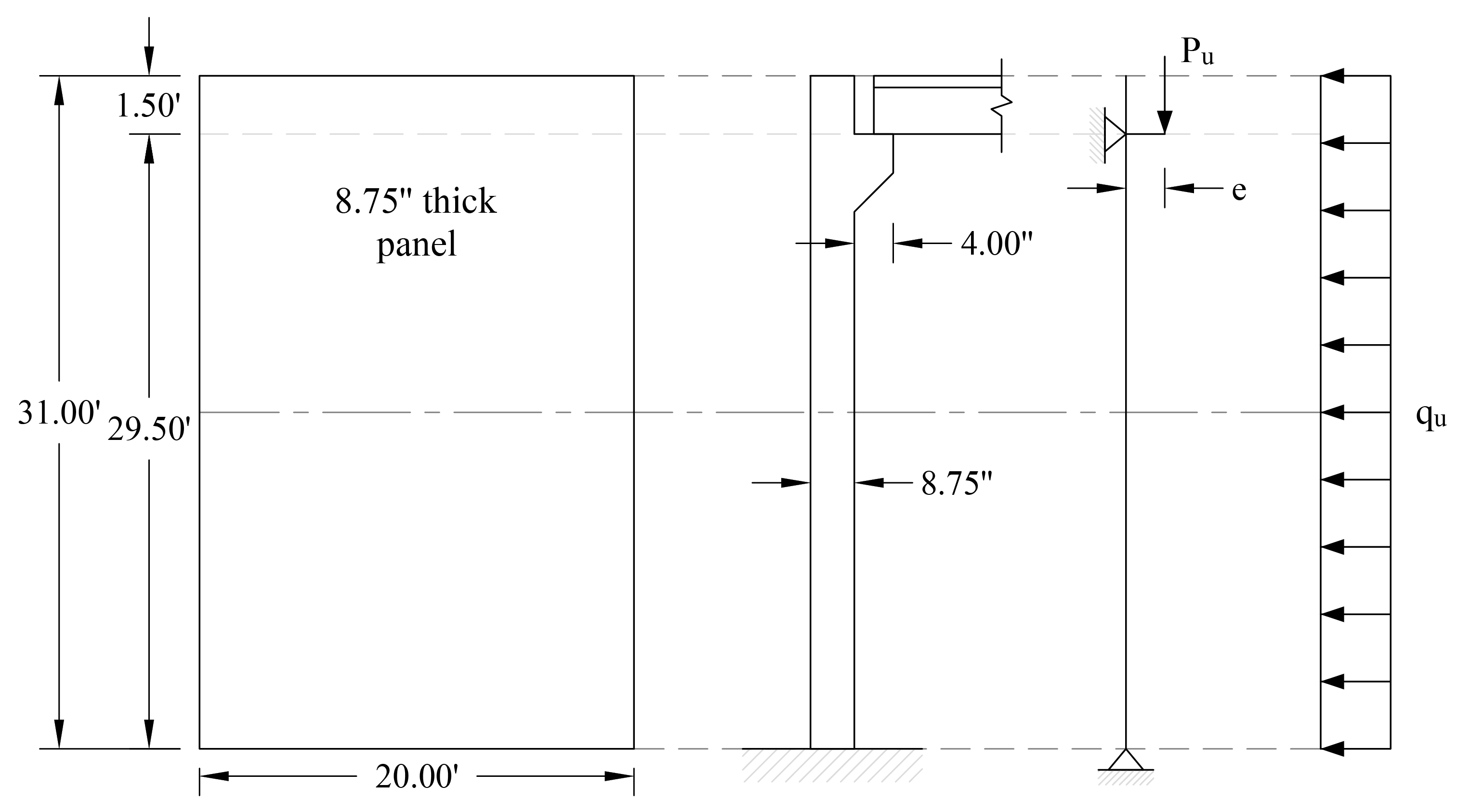
Figure 8.1 - Concrete Wall Geometry

8.1.2. Preparing the Input

1. From the Start screen, select New Project.

2. In the Main Program Window, select Project from the Ribbon.

• Select the DESIGN CODE, UNIT SYSTEM, and enter the PROJECT NAME and PROJECT DESCRIPTION.

3. From the Ribbon, select Grid.

• Click on the Generate in the left panel to have the program surface the following:

• Place a check mark in the X - VERTICAL box and enter the following values in the corresponding text boxes:

• Place a check mark in the Y - VERTICAL box and enter the following values in the corresponding text boxes:

• Click on the GENERATE button to return to the main window. Notice how the VERTICAL and HORIZONTAL grid lines now appear in the VIEWPORT.

4. From the Ribbon, select Define, then choose Plates from Objects to display the Plates dialog box.

• Input Plate-A for LABEL and 8.75 in. for THICKNESS.

• Click on the APPLY button to apply the changes.

5. Click on Concrete from Properties to display the Concrete dialog box.

• Enter the following:

• Click on the APPLY button to apply the changes.

6. Click on Reinforcement from Properties to display the Reinforcement dialog box.

• Enter the following:

• Click on the APPLY button to apply the changes.

7. Click on Plate Cracking Coefficient from Properties to display the Plate Cracking Coefficient dialog box.

• Enter the following:

• Click on the APPLY button to apply the changes.

8. Click on Plate Design Criteria from Properties to display the Plate Design Criteria dialog box.

• Enter the following:

• Click on the APPLY button to apply the changes.

9. Click on Supports from Restraints to display the Supports dialog box.

• Enter the following:

• Click on the APPLY button to apply the changes.

10. Click on Load Cases from Load Case/Combo. to display the Load Cases dialog box.

• Enter the following:

• Check SELF WEIGHT for CASE A.

• Click on the APPLY button to apply the changes.

11. Click on Service Load Combinations from Load Case/Combo. to display the Service Load Combinations dialog box.

• Enter the following service load combinations shown in the figure below:

12. Click on Ultimate Load Combinations from Load Case/Combo. to display the Ultimate Load Combinations dialog box.

• Enter the following load combinations shown in the figure below:

8.1.3. Assigning Properties

13. From the Ribbon, select Plates command.

• In the left panel, select Rectangle option then select PLATE-A from LABEL.

• In the VIEWPORT, marquee-select the region (A, 0) - (B, 2) to apply the selected plate to the entire wall.

8.1.4. Assigning Supports

14. From the Ribbon, select Stiffeners command.

• In the left panel, select Null.

• Apply at the bottom of the wall as shown in the figure below.

• Apply also on Axis 1 as shown in the figure below.

15. From the Ribbon, select Restraints command.

• In the left panel, select Linear then select HINGED from LABEL.

• Apply HINGED support to the bottom null stiffener as shown in the figure below.

• Select LATERAL from LABEL.

• Apply LATERAL support to the top null stiffener as shown in the figure below.

8.1.5. Assigning Loads

16. From the Ribbon, select Loads command.

• In the left panel, select Uniform Line then select A-DL from LOAD CASE and enter the following:

• Apply to the top null stiffener as shown in the figure below.

• Select B-LL from LOAD CASE and enter the following:

• Apply to the top null stiffener as shown in the figure below.

• In the left panel, select Uniform Area then select C-W from LOAD CASE and enter the following:

• Apply to the entire wall as shown in the figure below.

• Also, you can click on the 3D VIEW icon from View Controls (top right of the active viewport) to get a better view of the applied load.

8.1.6. Solving

17. From the Ribbon, select Solve command.

For Solve Options:

• Select ANALYSIS & DESIGN for RUN OPTIONS.

• Select YES for INCLUDED SECOND ORDER EFFECTS.

• Select DISABLE for MAXIMUM ALLOWED OUT-OF-PLANE DEFLECTION.

For Mesh Options:

• Enter 1.00 ft for the MAXIMUM ALLOWED MESH SIZE.

• Click on the Run button.

• The spWall Solver window is displayed and the solver messages are listed. After the solution is done, the design will be performed and then the focus will immediately be passed to the Results scope.

8.1.7. Viewing and Printing Results

18. After a successful run, results can be viewed in a contour form by selecting the Contours option from the left panel.

Please be advised that spWall displays the total flexure reinforcement, for each element, for two curtains of reinforcement.

19. Results can be viewed in a force diagram form by selecting the Diagrams option from the left panel.

20. Results can be also viewed in table format by selecting the Tables command from the Ribbon.

21. Results can be printed or exported in different formats by selecting the Reporter command from the Ribbon.