3.47Solve Model
After inputting the model geometry and defining the loads, the solution process can be started. From the Analyze menu, select Solve. The dialog box of Figure 3-36 appears. In the dialog box you may choose between several options.
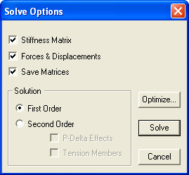
Figure 3-36 Solve Options dialog box
Selecting this option instructs the solver to calculate the member stiffness matrices as well as the global stiffness matrix of the entire structure. This option must be selected if solving the problem for the first time or if, after solving the problem, joints, members, or their assignments and definitions have been edited. However, if, after solving the problem, loads or load combinations are changed, the option need not be selected since the stiffness matrix will not be affected by the changes.
3.47.2Forces and Displacements
This option instructs the solver to calculate the load and displacement matrices. Joint displacements and reactions, along with the member end forces, will be computed as well.
This option instructs the program to save the matrices on disk. spFrame keeps all input data and solution results in memory (if possible) for fast execution and presentation. The size of a data file containing the stiffness matrices can be very large. You have to make sure that you have enough room on your disk to store it.
If the geometry, joint, member properties, and definitions of the model do not change, and the matrices were saved at run time, you can solve the structure at a future time, under a different set of loads or load combinations, by selecting the FORCES & DISPLACEMENTS option. This reduces the amount of time needed to solve the problem significantly.
FIRST ORDER option is the only available choice when executing the solver for the first time for a particular problem. Second order calculations require certain values from the first order solution. Therefore, to include the P-Δ effects or solve for tension members, the problem must be solved with the FIRST ORDER option first, then solved again with the SECOND ORDER option.
•In the SECOND ORDER option, P-Δ EFFECTS and/or TENSION MEMBERS option may be selected.
•To optimize the solution and minimize the bandwidth, choose the OPTIMIZE button. The dialog of Figure 3-37 appears.
•Select the AUTOMATIC option to let the program calculate the starting joint for optimization.
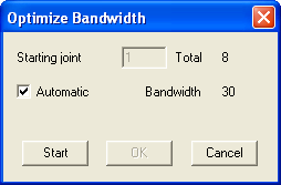
Figure 3-37 Optimize Bandwidth dialog box
•Clear the AUTOMATIC option to input an optimization starting joint in the corresponding text box.
•Choose the START button to start the optimization process. The resulting bandwidth is displayed.
•Choose the OK button to accept the optimization, or CANCEL otherwise.
Note that joint renumbering due to optimization is internal and does not affect the defined joint labels.
•After selecting the solver options, choose SOLVE. The spFrame program minimizes to an icon and the spFrame Solver window (shown in Figure 3-38) is displayed. The status box displays messages about the solution process and its progress. Should any errors or instabilities be encountered, they are also displayed. You can scroll through the messages displayed using the scroll bars at the side of the Solver window.
•To pause the solution process, choose the SUSPEND button. Your can then choose to cancel the solution process or continue by choosing the corresponding command button.
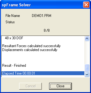
Figure 3-38 spFrame Solver Window
When the solver is done, choose the CLOSE button to start the LOCAL PROCESS. LOCAL PROCESS will process all elements and close automatically.