The PCA approach described below was developed as an extension of the Bresler Load Contour Method. The Bresler interaction equation was chosen as the most viable method in terms of accuracy, practicality, and simplification potential.
A typical Bresler load contour for a certain Pn is shown in the following "Figure 12 - Load Contour of Failure Surface S3 along Plane of Constant Pn". In the PCA method, point B is defined such that the nominal biaxial moment strengths Mnx and Mny at this point are in the same ratio as the uniaxial moment strengths Mnox and Mnoy. Therefore, at point B (Mnx / Mny = Mnox / Mnoy).
Figure 12 - Load Contour of Failure Surface S3 along Plane of Constant Pn
When the load contour of "Figure 12 - Load Contour of Failure Surface S3 along Plane of Constant Pn" is nondimensionalized, it takes the form shown in "Figure 13 - Nondimensional Load Contour at Constant Pn", and the point B will have x and y coordinates of β. When the bending resistance is plotted in terms of the dimensionless parameters Pn/Po, Mnx/Mnox, Mny/Mnoy (the latter two designated as the relative moments), the generated failure surface S4 (Pn/Po, Mnx/Mnox, Mny/Mnoy) assumes the typical shape shown in "Figure 14 - Nondimensional Load Contour at Constant Pn". The advantage of expressing the behavior in relative terms is that the contours of the surface ("Figure 13 - Nondimensional Load Contour at Constant Pn") - i.e., the intersection formed by planes of constant Pn/Po and the surface - can be considered for design purposes to be symmetrical about the vertical plane bisecting the two coordinate planes. Even for sections that are rectangular or have unequal reinforcement on the two adjacent faces, this approximation yields values sufficiently accurate for design.
Figure 13 - Nondimensional Load Contour at Constant Pn
Figure 14 - Nondimensional Load Contour at Constant Pn
The reference obtained the relationship between α from Eq. (10) and β by substituting the coordinates of point B from "Figure 11 - Interaction Curves for Bresler Load Contour Method" into Eq. (10), and solving for α in terms of β. This yields:

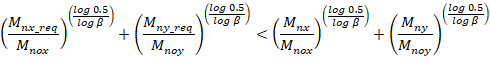
Thus, Eq. (10) may be written as:

For design convenience, a plot of the curves generated by Eq. (14) for nine values of β are given in "Figure 15 - Biaxial Moment Strength Relationship". Note that when β = 0.5, its lower limit, Eq. (14) is a straight line joining the points at which the relative moments equal 1.0 along the coordinate planes. When β = 1.0, its upper limit, Eq. (14) is two lines, each of which is parallel to one of the coordinate planes.
Figure 15 - Biaxial Moment Strength Relationship
β is dependent primarily on the ratio Pn/Po and to a lesser, though still significant extent, on the bar arrangement, the reinforcement index ω and the strength of the reinforcement as shown in "Figure 16 - Biaxial Design Constants".
Figure 16 - Biaxial Design Constants
Rapid and easy convergence to a satisfactory section can be achieved by approximating the curves in "Figure 15 - Biaxial Moment Strength Relationship" by two straight lines intersecting at the 45º line, as shown in "Figure 17 - Bilinear Approximation of Nondimensionalized Load Contour".
Figure 17 - Bilinear Approximation of Nondimensionalized Load Contour
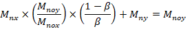
By simple geometry, it can be shown that the equation of the upper lines is:

which can be restated for design convenience as follows:
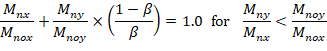
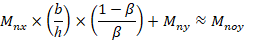
For rectangular sections with reinforcement equally distributed on all faces, Eq. (16) can be approximated by:
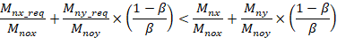
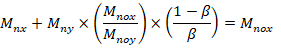
The equation of the lower line of "Figure 17 - Bilinear Approximation of Nondimensionalized Load Contour" is:

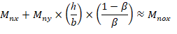
For rectangular sections with reinforcement equally distributed on all faces,
In design Eqs. (17) and (20), the ratio b/h or h/b must be chosen and the value of β must be assumed. For lightly loaded columns, β will generally vary from 0.55 to about 0.70. Hence, a value of 0.65 for β is generally a good initial choice in a biaxial bending analysis.
Po, Mnox, Mnoy and β need to be determined to use this method:
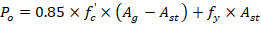

Since the section is symmetrical:
 ("Figure 6 - Column Section Capacity Interaction Diagram (spColumn)")
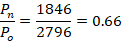
β can be determined using Po, ρg and the biaxial design constants figure:
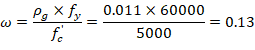 , where
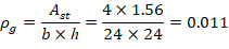
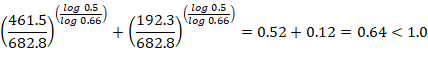
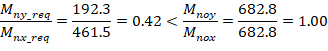
β = 0.66 ("Figure 18 - Biaxial Design Constants (4 Bar Arrangement)"):
Figure 18 - Biaxial Design Constants (4 Bar Arrangement)
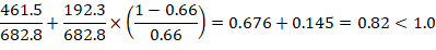
Using the accurate equation (equation 14):